Note
This example is available as a jupyter notebook here.
With the release of imt-ring >= v1.7.0, a CLI tool ring-view has been added.
>$ ring-view --help
NAME
    ring-view - View motion given by trajectory of minimal coordinates in interactive viewer.

SYNOPSIS
    ring-view PATH_SYS_XML <flags>

DESCRIPTION
    View motion given by trajectory of minimal coordinates in interactive viewer.

POSITIONAL ARGUMENTS
    PATH_SYS_XML
        Type: str
        Path to xml file defining the system.

FLAGS
    -p, --path_qs_np=PATH_QS_NP
        Type: Optional[Optional]
        Default: None
        Path to numpy array containing the timeseries of minimal coordinates with shape (T, DOF) where DOF is equal to `sys.q_size()`. Each minimal coordiante is from parent to child. So for example a `spherical` joint that connects the first body to the worldbody has a minimal coordinate of a quaternion that gives from worldbody to first body. The sampling rate of the motion is inferred from the `sys.dt` attribute. If `None` (default), then simply renders the unarticulated pose of the system.
    Additional flags are accepted.
Suppose, we have the following system stored in pendulum.xml
<x_xy model="double_pendulum">
<options dt="0.01" gravity="0 0 9.81"></options>
<worldbody>
<body damping="2" euler="0 90 0" joint="ry" name="upper" pos="0 0 2">
<geom dim="1 0.25 0.2" mass="10" pos="0.5 0 0" type="box"></geom>
<body damping="2" joint="ry" name="lower" pos="1 0 0">
<geom dim="1 0.25 0.2" mass="10" pos="0.5 0 0" type="box"></geom>
</body>
</body>
</worldbody>
</x_xy>
Then, we can directly execute and create an interactive view of the system using ring-view pendulum.xml
Alternatively, we can also work with the InteractiveViewer class.
from ring.extras.interactive_viewer import InteractiveViewer
import ring
sys = ring.System.create("""
<x_xy model="double_pendulum">
<options dt="0.01" gravity="0 0 9.81"></options>
<worldbody>
<body damping="2" euler="0 90 0" joint="ry" name="upper" pos="0 0 2">
<geom dim="1 0.25 0.2" mass="10" pos="0.5 0 0" type="box"></geom>
<body damping="2" joint="ry" name="lower" pos="1 0 0">
<geom dim="1 0.25 0.2" mass="10" pos="0.5 0 0" type="box"></geom>
</body>
</body>
</worldbody>
</x_xy>
""")
viewer = InteractiveViewer(sys)

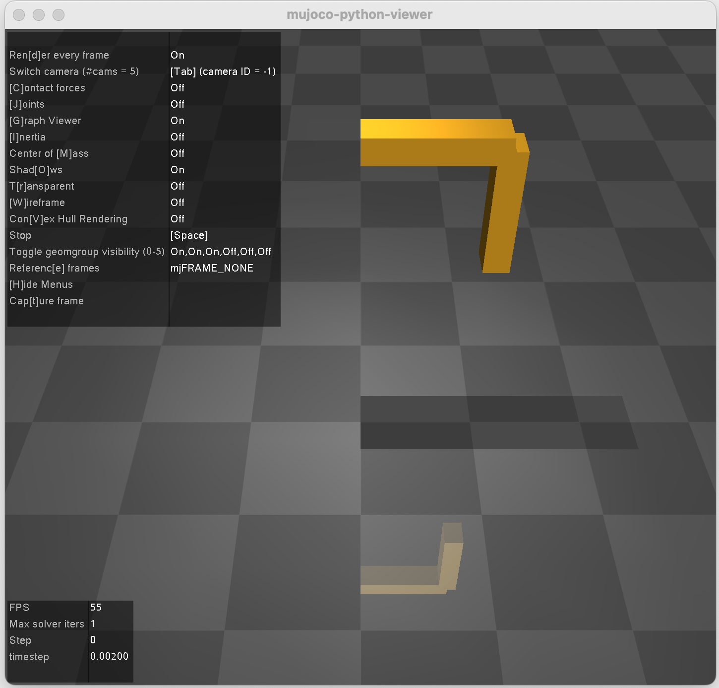
Notice how this opens the interactive viewer window (where you can use the mouse to navigate, without blocking the main thread). So, we can update the view from this notebook.
import numpy as np
viewer.update_q(np.array([-np.pi / 2, np.pi / 2]))
This is really powerful for creating virtually any animation.